Surface Integrals Benchmark using Gauss-Bonnet Theorem
Overview
This document outlines a comprehensive benchmark for the computation of surface integrals utilizing the high-order volume elements (HOVE) algorithm, specifically tailored for algebraic varieties.
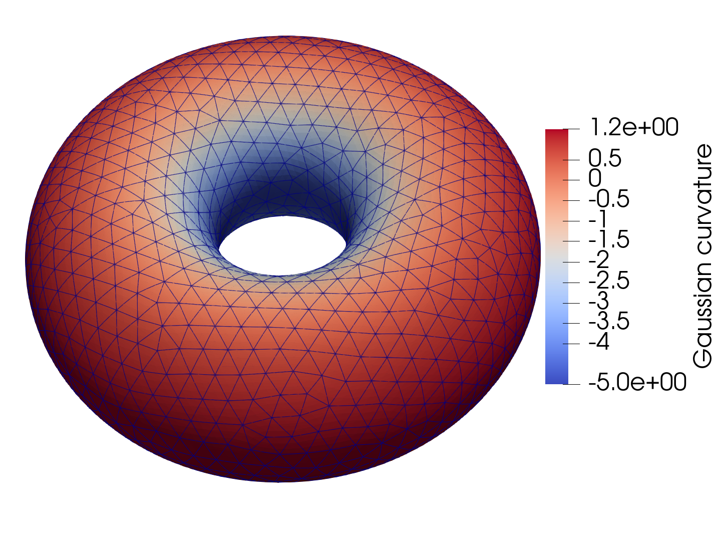
Gauss-Bonnet Theorem on Torus
The Gauss-Bonnet Theorem establishes that the integral of Gaussian curvature over a surface must satisfy the equation:
where \(\chi(\mathcal{M})\) denotes the Euler Characteristic of the surface.
For a torus, with \(\chi(\mathcal{M}) = 0\), the theorem simplifies to:
Imports
import matplotlib.pyplot as plt
import numpy as np
from math import pi
from time import time

# Local imports
import surfgeopy as sp
mesh_path1 = "../meshes/torus_496.mat"
mesh_path2 = "../meshes/torus_1232.mat"

R = 2
r = 1

def phi(x: np.ndarray):
    ph = np.sqrt(x[0]*x[0] + x[1]*x[1])
    return (ph - R)*(ph - R) + x[2]*x[2] - r*r

def dphi(x: np.ndarray):
    ph = np.sqrt(x[0]*x[0] + x[1]*x[1])
    return np.array([-2*R*x[0]/ph + 2*x[0], -2*R*x[1]/ph + 2*x[1], 2*x[2]])

def fun_1(x: np.ndarray):
    t1 = np.sqrt(x[0]*x[0] + x[1]*x[1])
    t2 = (t1 - 2) / 1
    return t2 / (1*t1)
Error Evaluation Function
def err_g(intp_degree, lp_degree, mesh_path, refinement):
    t0 = time()
    areas = sp.integration(phi, dphi, mesh_path, intp_degree, lp_degree, refinement, fun_1)
    t1 = time()
    sum_area = sum(areas)
    t1 = time()
    exact_area = 0
    print("Absolute error: ", abs(sum_area - exact_area))
    print("The main function takes:", {(t1-t0)})
    error = abs(sum_area - exact_area)
    return error
Degree of Polynomial
Nrange = list(range(2, 18))
lp_degree = float("inf")
error1 = []
refinement = 0

for n in Nrange:
    if n % 1 == 0:
        print(n)
    erro1 = err_g(n, lp_degree, mesh_path2, refinement)
    error1.append(erro1)
Result Visualization
plt.semilogy(Nrange, error1, '-or')
plt.xlabel("Polynomial degree", fontsize=13)
plt.ylabel("Absolute error", fontsize=13)
plt.xticks(np.arange(min(Nrange), max(Nrange)+1, 1.0))
plt.ylim([1.0e-17, 2.0e-03])
plt.grid()
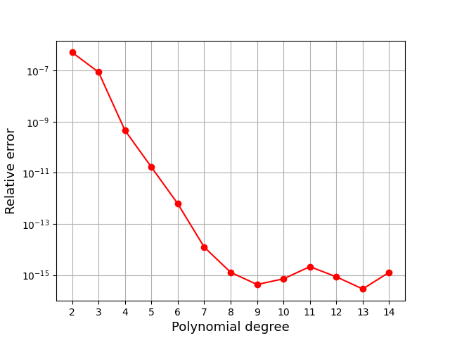
Gauss Bonnet theorem on a Genus 2 Surface
For a genus two surface, the Euler Characteristic is \(\chi(\mathcal{M}) = 2 - 2g\), where \((g)\) is the genus of the surface. Therefore, we have:
Imports
import matplotlib.pyplot as plt
import numpy as np
from math import pi
from time import time

# Local imports
import surfgeopy as sp

mesh_path = "../meshes/genus_two_N=15632.mat"

def phi(x: np.ndarray):
    return 2*x[1]*(x[1]*x[1] - 3*x[0]*x[0])*(1 - x[2]*x[2]) + (x[0]*x[0] + x[1]*x[1])**2 - (9*x[2]*x[2] - 1)*(1 - x[2]*x[2])


def dphi(x: np.ndarray):
    return np.array([4*x[0]*(x[0]*x[0] + x[1]*x[1] + 3*x[1]*(x[2]*x[2] - 1)),
                     4*x[1]*(x[0]*x[0] + x[1]*x[1]) + 4*x[1]*x[1]*(1 - x[2]*x[2]) + 2*(3*x[0]*x[0] - x[1]*x[1])*(x[2]*x[2] - 1),
                     4*x[2]*(x[1]*(3*x[0]*x[0] - x[1]*x[1]) + 9*x[2]*x[2] - 5)])
def fun_1(x: np.ndarray):
    return (4*1**2*(-900*(x[0]**2 + x[1]**2)*x[2]**2 + 45*1**10*(x[0]**2 + x[1]**2)*(-3*x[0]**2*x[1] + x[1]**3)**2*x[2]**6 -                6*1**3*x[1]*(-3*x[0]**2 + x[1]**2)*x[2]**2*(159*(x[0]**2 + x[1]**2) - 460*x[2]**2)+\
                                         15*1*x[1]*(-3*x[0]**2 + x[1]**2)*(9*(x[0]**2 + x[1]**2) - 40*x[2]**2) + 15*1**9*x[1]*(-3*x[0]**2 + x[1]**2)*x[2]**4*(3*x[0]**6 - 9*x[0]**4*x[1]**2 + 21*x[0]**2*x[1]**4 + x[1]**6 + 27*(x[0]**2 + x[1]**2)*x[2]**4) + \
                                         15*1**2*(3*(x[0]**6 + 21*x[0]**4*x[1]**2 - 9*x[0]**2*x[1]**4 + 3*x[1]**6) + 20*(x[0]**2 + x[1]**2)**2*x[2]**2 + 336*(x[0]**2 + x[1]**2)*x[2]**4) + 9*1**5*x[1]*(-3*x[0]**2 + x[1]**2)*(x[0]**6 + 21*x[0]**4*x[1]**2 - 9*x[0]**2*x[1]**4 + 3*x[1]**6 + 212*(x[0]**2 + x[1]**2)*x[2]**4 - 456*x[2]**6) + \
                                         1**4*(-20*x[0]**8 + 163*x[0]**6*x[1]**2 - 39*x[0]**4*x[1]**4 - 215*x[0]**2*x[1]**6 + 7*x[1]**8 - 3*(171*x[0]**6 + 2151*x[0]**4*x[1]**2 - 579*x[0]**2*x[1]**4 + 353*x[1]**6)*x[2]**2 - 1080*(x[0]**2 + x[1]**2)**2*x[2]**4 - 10296*(x[0]**2 + x[1]**2)*x[2]**6) + \
                                         3*1**6*x[2]**2*(3*(x[0]**2 + x[1]**2)*(12*x[0]**6 + 27*x[0]**4*x[1]**2 + 42*x[0]**2*x[1]**4 + 11*x[1]**6) + (345*x[0]**6 + 3213*x[0]**4*x[1]**2 - 417*x[0]**2*x[1]**4 + 587*x[1]**6)*x[2]**2 + 324*(x[0]**2 + x[1]**2)**2*x[2]**4 + 3024*(x[0]**2 + x[1]**2)*x[2]**6) - \
                                         2*1**7*x[1]*(-3*x[0]**2 + x[1]**2)*(2*(x[0]**2 + x[1]**2)**4 + 3*(9*x[0]**6 + 9*x[0]**4*x[1]**2 + 39*x[0]**2*x[1]**4 + 7*x[1]**6)*x[2]**2 + 747*(x[0]**2 + x[1]**2)*x[2]**6 - 972*x[2]**8) + 3*1**8*x[2]**2*(-4*(x[0]**2 + x[1]**2)**2*(3*x[0]**6 - 9*x[0]**4*x[1]**2 + \
                                         21*x[0]**2*x[1]**4 + x[1]**6) - 21*x[1]**2*(-3*x[0]**2 + x[1]**2)**2*(x[0]**2 + x[1]**2)*x[2]**2 - 9*(21*x[0]**6 + 153*x[0]**4*x[1]**2 + 3*x[0]**2*x[1]**4 + 31*x[1]**6)*x[2]**4 - 972*(x[0]**2 + x[1]**2)*x[2]**8)))/(100*x[2]**2 - 12*1**5*x[1]*(-3*x[0]**2 + x[1]**2)*x[2]**2*(x[0]**2 + x[1]**2 + 6*x[2]**2) + \
                                         4*1**3*x[1]*(-3*x[0]**2 + x[1]**2)*(3*(x[0]**2 + x[1]**2) + 10*x[2]**2) + 1**6*x[2]**2*(4*(-3*x[0]**2*x[1] + x[1]**3)**2 + 9*(x[0]**2 + x[1]**2)**2*x[2]**2) + 9*1**2*((x[0]**2 + x[1]**2)**2 - 40*x[2]**4) + 2*1**4*(2*(x[0]**2 + x[1]**2)**3 - 9*(x[0]**2 + x[1]**2)**2*x[2]**2 + 162*x[2]**6))**2
Error Evaluation Function
def err_g(intp_degree, lp_degree, mesh_path, refinement):
    t0 = time()
    areas = sp.integration(phi, dphi, mesh_path, intp_degree, lp_degree, refinement, fun_1)
    t1 = time()
    sum_area = sum(areas)
    t1 = time()
    exact_area = -4*pi
    print("Relative error: ", abs((sum_area - exact_area) / exact_area))
    print("The main function takes:", {(t1-t0)})
    error = abs((sum_area - exact_area) / exact_area)
    return error
Degree of Polynomial
Nrange = list(range(2, 15))
lp_degree = float("inf")
error1 = []
refinement = 0
for n in Nrange:
    if n % 1 == 0:
        print(n)
    erro1 = err_g(n, lp_degree, mesh_path, refinement)
    error1.append(erro1)
Result Visualization
plt.semilogy(Nrange, error1, '-or')
plt.xlabel("Polynomial degree", fontsize=13)
plt.ylabel("Relative error", fontsize=13)
plt.xticks(np.arange(min(Nrange), max(Nrange)+1, 1.0))
plt.grid()
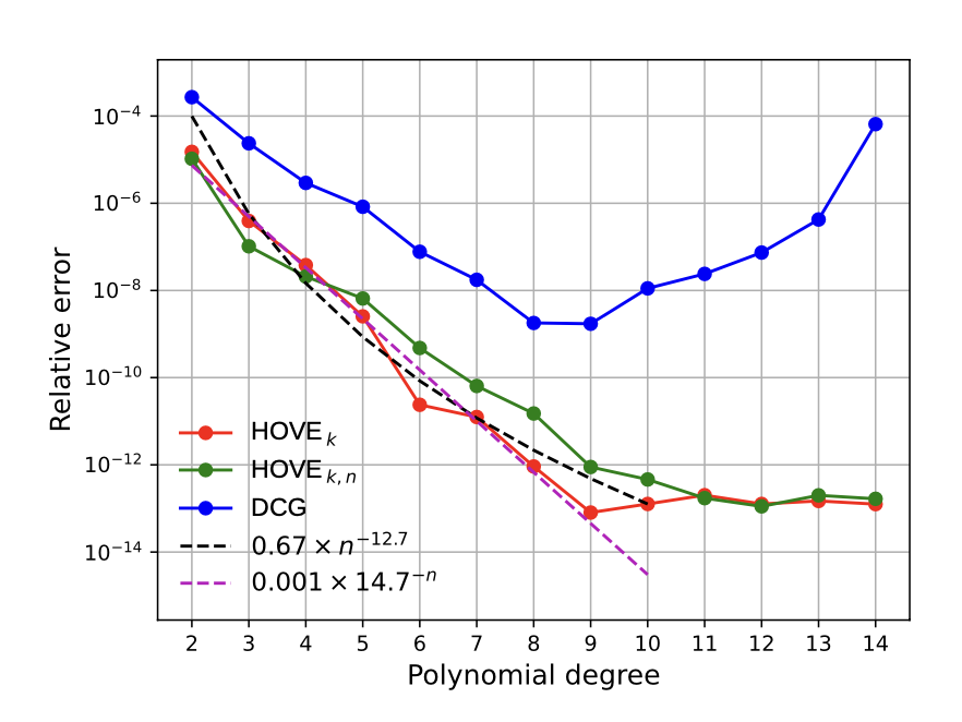
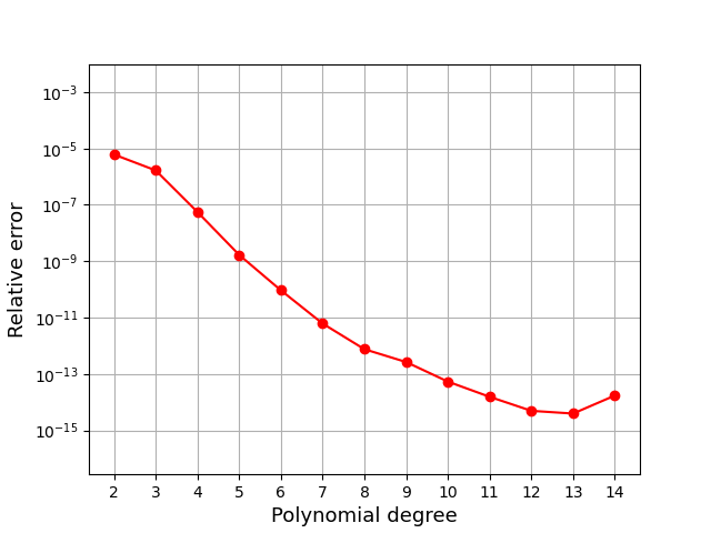
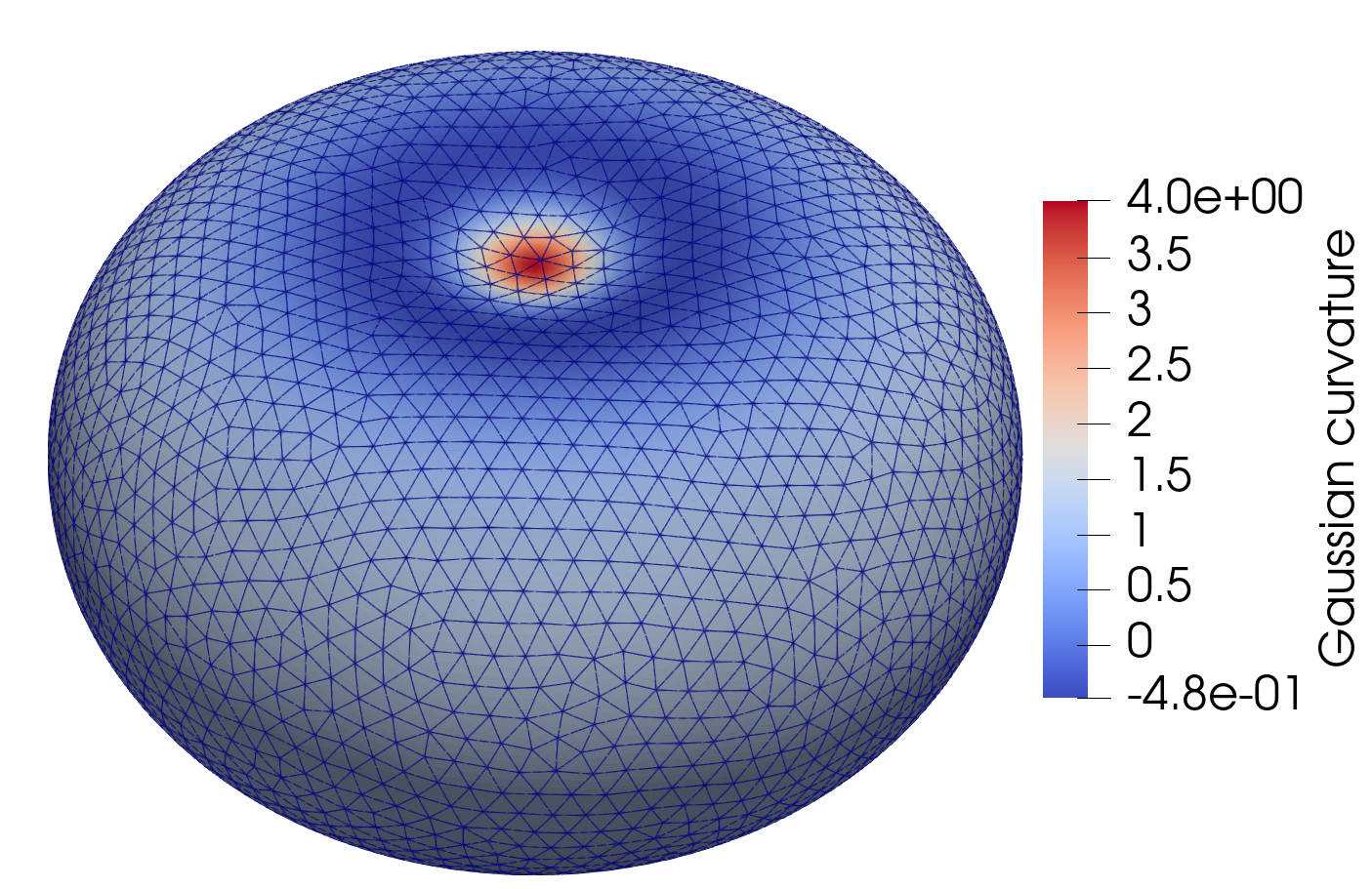
Gauss Bonnet theorem on ellipsoid
For an oblate spheroid, that is an ellipsoid where \((a = b > c)\), the Euler Characteristic is \(\chi(\mathcal{M}) = 2\), therefore we have:

Imports
import matplotlib.pyplot as plt
import numpy as np
from math import pi
from time import time

# Local imports
import surfgeopy as sp

mesh_path ="../meshes/ellipsoid_N=4024_a=0.6_b=0.8_c=2.mat"
a=0.6
b=0.8
c=2.0

def phi(x: np.ndarray):
    return (x[0]**2/a**2 + x[1]**2/b**2 + x[2]**2/c**2) - 1

def dphi(x: np.ndarray):
    return np.array([2*x[0]/a**2, 2*x[1]/b**2, 2*x[2]/c**2])

def fun_1(x: np.ndarray):
    return 1.0 / (((a*b*c)**2) * (x[0]**2/(a**4) + x[1]**2/(b**4) + x[2]**2/(c**4))**2)
Error Evaluation Function
def err_g(intp_degree, lp_degree, mesh_path, refinement):
    t0 = time()
    areas = sp.integration(phi, dphi, mesh_path, intp_degree, lp_degree, refinement, fun_1)
    t1 = time()
    sum_area = sum(areas)
    t1 = time()
    exact_area = 4*pi
    print("Relative error: ", abs((sum_area - exact_area)/exact_area))
    print("The main function takes:", {(t1-t0)})
    error = abs((sum_area - exact_area)/exact_area)
    time_s = t1 - t0
    return error, time_s
Degree of Polynomial
Nrange = list(range(2, 27))
lp_degree = float("inf")
error1 = []
execution_times = []
refinement = 0
for n in Nrange:
    if n % 1 == 0:
        print(n)
    erro1, times = err_g(n, lp_degree, mesh_path, refinement)
    error1.append(erro1)
    execution_times.append(times)
Result Visualization
plt.semilogy(Nrange, error1, '-or')
plt.xlabel("Polynomial degree", fontsize=13)
plt.ylabel("Relative error", fontsize=13)
plt.xticks(np.arange(min(Nrange), max(Nrange)+1, 1.0))
plt.grid()
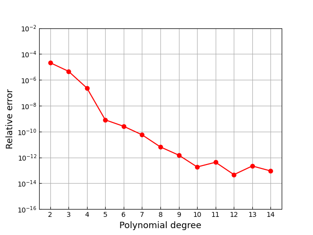
Gauss Bonnet theorem on the first Dziuk’s surface
Consider the Dzikus surface with implicit equation as:
the Euler Characteristic is \(\chi(\mathcal{M})=2\), therefore we have:

Imports
import matplotlib.pyplot as plt
import numpy as np
from math import pi
from time import time

# Local imports
import surfgeopy as sp

mesh_path = "../meshes/dziukmesh_N=8088.mat"

def phi(x: np.ndarray):
    return (x[0] - x[2]**2)**2 + x[1]**2 + x[2]**2 - 1

def dphi(x: np.ndarray):
    return np.array([2*(x[0] - x[2]**2), 2*x[1], 2*(-2*x[0]*x[2] + 2*x[2]**3 + x[2])])

def fun_1(x: np.ndarray):
    return (x[1]**2 + x[2]**2 - (x[0] - x[2]**2)*(x[0]*(2*x[0]-1) + 2*x[1]**2 + x[2]**2 - 4*x[0]*x[2]**2 + 2*x[2]**4)) / (x[1]**2 + x[2]**2 + (x[0] - x[2]**2)*(x[0] + (4*x[0]-5)*x[2]**2 - 4*x[2]**4))**2
Error Evaluation Function
def err_g(intp_degree, lp_degree, mesh_path, refinement):
    t0 = time()
    areas = sp.integration(phi, dphi, mesh_path, intp_degree, lp_degree, refinement, fun_1)
    t1 = time()
    sum_area = sum(areas)
    t1 = time()
    exact_area = 4*pi
    print("Relative error: ", abs((sum_area - exact_area)/exact_area))
    print("The main function takes:", t1 - t0)
    error = abs((sum_area - exact_area)/exact_area)
    return error
Degree of Polynomial
Nrange = list(range(2, 15))
lp_degree = float("inf")
error1 = []
refinement = 0
for n in Nrange:
    if n % 1 == 0:
        print(n)
    erro1 = err_g(n, lp_degree, mesh_path, refinement)
    error1.append(erro1)
Result Visualization
plt.semilogy(Nrange, error1, '-or')
plt.xlabel("Polynomial degree", fontsize=13)
plt.ylabel("Relative error", fontsize=13)
plt.xticks(np.arange(min(Nrange), max(Nrange)+1, 1.0))
plt.ylim([1.0e-16, 1.0e-02])
plt.grid()
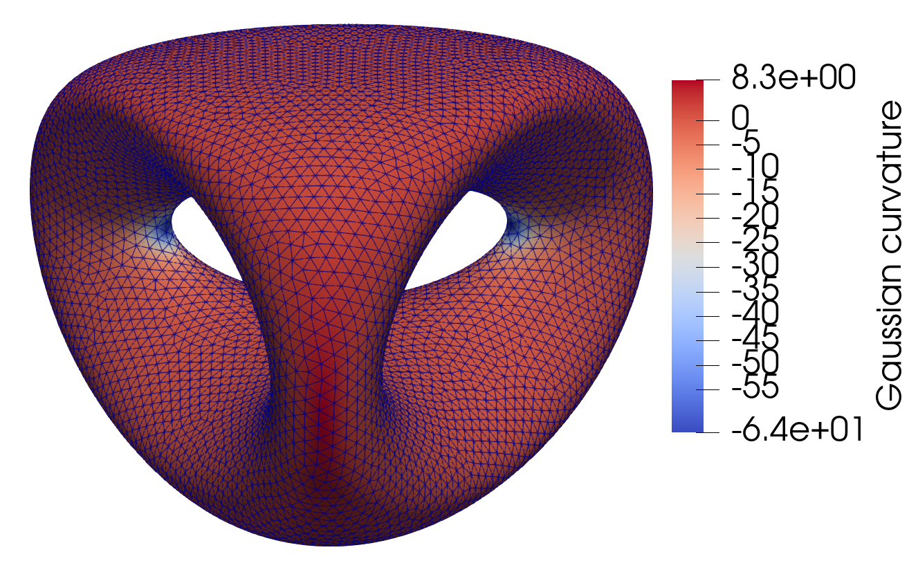
Gauss Bonnet theorem on Bioconcave surface
Consider the bioconcave surface with the implicit equation:
The Euler Characteristic is \(\chi(\mathcal{M})=2\), therefore we have:
import matplotlib.pyplot as plt
import numpy as np
from math import pi
from time import time

# Local imports
import surfgeopy as sp

mesh_path ="../meshes/bioconcave_N=5980.mat"

d = 0.80
c = -0.9344

def phi(x: np.ndarray):
    return (d**2 + x[0]**2 + x[1]**2 + x[2]**2)**3 - 8*d**2*(x[1]**2 + x[2]**2) - c**4

def dphi(x: np.ndarray):
    return np.array([6*x[0]*(d**2 + x[0]**2 + x[1]**2 + x[2]**2)**2,
                     6*x[1]*(d**2 + x[0]**2 + x[1]**2 + x[2]**2)**2 - 16*d**2*x[1],
                     6*x[2]*(d**2 + x[0]**2 + x[1]**2 + x[2]**2)**2 - 16*d**2*x[2]])

def fun_1(x: np.ndarray):
    return (6*(d**2 + x[0]**2 + x[1]**2 + x[2]**2)* \
         ((-16*d**2*x[2] + 6*x[2]*(d**2 + x[0]**2 + x[1]**2 + x[2]**2)**2)* \
            (24*x[0]**2*x[2]*(d**2 + x[0]**2 + x[1]**2 + x[2]**2)**2* \
               (16*d**2 - 6*(d**2 + x[0]**2 + x[1]**2 + x[2]**2)**2) - \
              24*x[1]*x[2]*(d**2 + x[0]**2 + x[1]**2 + x[2]**2)**2* \
               (-16*d**2*x[1] + 6*x[1]*(d**2 + x[0]**2 + x[1]**2 + x[2]**2)**2) + \
              (-16*d**2*x[2] + 6*x[2]*(d**2 + x[0]**2 + x[1]**2 + x[2]**2)**2)* \
               (-96*x[0]**2*x[1]**2*(d**2 + x[0]**2 + x[1]**2 + x[2]**2) + \
                 (d**2 + 5*x[0]**2 + x[1]**2 + x[2]**2)* \
                  (-16*d**2 + 24*x[1]**2*(d**2 + x[0]**2 + x[1]**2 + x[2]**2) + \
                    6*(d**2 + x[0]**2 + x[1]**2 + x[2]**2)**2))) + \
           (-16*d**2*x[1] + 6*x[1]*(d**2 + x[0]**2 + x[1]**2 + x[2]**2)**2)* \
            (24*x[0]**2*x[1]*(d**2 + x[0]**2 + x[1]**2 + x[2]**2)**2* \
               (16*d**2 - 6*(d**2 + x[0]**2 + x[1]**2 + x[2]**2)**2) -  \
              24*x[1]*x[2]*(d**2 + x[0]**2 + x[1]**2 + x[2]**2)**2* \
               (-16*d**2*x[2] + 6*x[2]*(d**2 + x[0]**2 + x[1]**2 + x[2]**2)**2) + \
              (-16*d**2*x[1] + 6*x[1]*(d**2 + x[0]**2 + x[1]**2 + x[2]**2)**2)* \
               (-96*x[0]**2*x[2]**2*(d**2 + x[0]**2 + x[1]**2 + x[2]**2) + \
                 (d**2 + 5*x[0]**2 + x[1]**2 + x[2]**2)* \
                  (-16*d**2 + 24*x[2]**2*(d**2 + x[0]**2 + x[1]**2 + x[2]**2) +  \
                    6*(d**2 + x[0]**2 + x[1]**2 + x[2]**2)**2))) +  \
           6*x[0]**2*(d**2 + x[0]**2 + x[1]**2 + x[2]**2)**2* \
            (4*x[1]*(16*d**2 - 6*(d**2 + x[0]**2 + x[1]**2 + x[2]**2)**2)* \
               (-16*d**2*x[1] + 6*x[1]*(d**2 + x[0]**2 + x[1]**2 + x[2]**2)**2) +  \
              4*x[2]*(16*d**2 - 6*(d**2 + x[0]**2 + x[1]**2 + x[2]**2)**2)* \
               (-16*d**2*x[2] + 6*x[2]*(d**2 + x[0]**2 + x[1]**2 + x[2]**2)**2) + \
              (d**2 + x[0]**2 + x[1]**2 + x[2]**2)* \
               (-576*x[1]**2*x[2]**2*(d**2 + x[0]**2 + x[1]**2 + x[2]**2)**2 + \
                 (-16*d**2 + 24*x[1]**2*(d**2 + x[0]**2 + x[1]**2 + x[2]**2) + \
                    6*(d**2 + x[0]**2 + x[1]**2 + x[2]**2)**2)* \
                  (-16*d**2 + 24*x[2]**2*(d**2 + x[0]**2 + x[1]**2 + x[2]**2) +  \
                    6*(d**2 + x[0]**2 + x[1]**2 + x[2]**2)**2)))))/ \
           (36*x[0]**2*(d**2 + x[0]**2 + x[1]**2 + x[2]**2)**4 +  \
              (16*d**2*x[1] - 6*x[1]*(d**2 + x[0]**2 + x[1]**2 + x[2]**2)**2)**2 +  \
              (16*d**2*x[2] - 6*x[2]*(d**2 + x[0]**2 + x[1]**2 + x[2]**2)**2)**2)**2
Error Evaluation Function
def err_g(intp_degree, lp_degree, mesh_path, refinement):
    t0 = time()
    areas = sp.integration(phi, dphi, mesh_path, intp_degree, lp_degree, refinement, fun_1)
    t1 = time()
    sum_area = sum(areas)
    t1 = time()
    exact_area = 4*pi
    print("Relative error: ", abs((sum_area - exact_area)/exact_area))
    print("The main function takes:", {(t1-t0)})
    error = abs((sum_area - exact_area)/exact_area)
    return error
Degree of Polynomial
Nrange = list(range(2, 15))
lp_degree = float("inf")
error1 = []
refinement = 0
for n in Nrange:
    if n % 1 == 0:
        print(n)
    erro1 = err_g(n, lp_degree, mesh_path, refinement)
    error1.append(erro1)
Result Visualization
plt.semilogy(Nrange, error1, '-or')
plt.xlabel("Polynomial degree", fontsize=13)
plt.ylabel("Relative error", fontsize=13)
plt.xticks(np.arange(min(Nrange), max(Nrange)+1, 1.0))
plt.grid()